Supervised learning¶

Binary classification of protein sequences¶

Proteins are polymers made of 20 different amino acids. Proteins have been classified into different families based on their sequence similarity. Positive and negative datasets corresponding to one of the protein families are available here

Extract features from the protein sequences

Amino Acid Composition refers to frequency of each amino acid within a protein sequence. E.g. if a protein has a sequence ‘MSAARQTTRKAE’ it’s amino acid composition can be represented as a vector of length 20:

‘A’:3,’C’:0,’D’:0,’E’:1,’F’:0,’G’:0,’H’:0,’I’:0,’K’:1,’L’:0,’M’:1,’N’:0,’P’:0,’Q’:1,’R’:1,’S’:1,’T’:2,’V’:0,’W’:0,’Y’:0

In this way any protein sequence can be represented as a feature vector of fixed length. This is important because the protein sequences, even within the same class, can have different number of amino acids.

import scipy
import numpy as np
import pandas as pd
import matplotlib.pyplot as plt
import seaborn as sns
from Bio import SeqIO
from Bio.SeqUtils.ProtParam import ProteinAnalysis
from sklearn import model_selection

positive_dict = SeqIO.to_dict(SeqIO.parse("positive-aars.fasta", "fasta"))
negative_dict = SeqIO.to_dict(SeqIO.parse("negative-aars.fasta", "fasta"))

## Amino acid composition calculation##
#c1 = ProteinAnalysis("AAAASTRRRTRRAWEQWERQW").count_amino_acids()
df1 = pd.DataFrame()
for keys,values in positive_dict.items():
    df1 = df1.append(pd.Series(ProteinAnalysis(str(values.seq)).get_amino_acids_percent(),name='1'))
for keys,values in negative_dict.items():
    df1 = df1.append(pd.Series(ProteinAnalysis(str(values.seq)).get_amino_acids_percent(),name='-1'))

print("Number of positive samples: ", len(positive_dict))
print("Number of negative samples: ", len(negative_dict))

df1

Number of positive samples:  117
Number of negative samples:  117

	A	C	D	E	F	G	H	I	K	L	M	N	P	Q	R	S	T	V	W	Y
1	0.035928	0.007984	0.041916	0.131737	0.055888	0.049900	0.017964	0.081836	0.119760	0.107784	0.015968	0.037924	0.037924	0.011976	0.037924	0.055888	0.049900	0.057884	0.013972	0.029940
1	0.076233	0.004484	0.049327	0.065770	0.029895	0.082212	0.020927	0.055306	0.082212	0.074738	0.040359	0.037369	0.043348	0.056801	0.058296	0.055306	0.061286	0.053812	0.017937	0.034380
1	0.093333	0.009524	0.068571	0.080000	0.026667	0.120000	0.024762	0.059048	0.055238	0.095238	0.028571	0.015238	0.041905	0.019048	0.074286	0.060952	0.020952	0.053333	0.009524	0.043810
1	0.079470	0.036424	0.052980	0.067881	0.046358	0.072848	0.023179	0.046358	0.021523	0.117550	0.019868	0.016556	0.046358	0.039735	0.081126	0.072848	0.049669	0.072848	0.008278	0.028146
1	0.084158	0.003300	0.046205	0.094059	0.034653	0.077558	0.018152	0.061056	0.089109	0.099010	0.036304	0.057756	0.031353	0.029703	0.026403	0.047855	0.042904	0.061056	0.011551	0.047855
...	...	...	...	...	...	...	...	...	...	...	...	...	...	...	...	...	...	...	...	...
-1	0.087221	0.004057	0.050710	0.060852	0.034483	0.068966	0.020284	0.056795	0.070994	0.089249	0.020284	0.036511	0.050710	0.042596	0.054767	0.079108	0.052738	0.075051	0.004057	0.040568
-1	0.067901	0.009259	0.049383	0.030864	0.027778	0.055556	0.024691	0.037037	0.030864	0.080247	0.015432	0.040123	0.111111	0.080247	0.104938	0.101852	0.058642	0.030864	0.018519	0.024691
-1	0.053521	0.010329	0.056338	0.101408	0.037559	0.037559	0.014085	0.059155	0.082629	0.110798	0.025352	0.059155	0.029108	0.047887	0.061033	0.078873	0.048826	0.046948	0.005634	0.033803
-1	0.038462	0.022869	0.070686	0.062370	0.062370	0.024948	0.014553	0.066528	0.060291	0.121622	0.016632	0.069647	0.027027	0.040541	0.050936	0.096674	0.061331	0.058212	0.009356	0.024948
-1	0.042791	0.014884	0.055814	0.071628	0.058605	0.032558	0.020465	0.053953	0.071628	0.110698	0.010233	0.054884	0.044651	0.042791	0.059535	0.102326	0.040930	0.054884	0.013023	0.043721

234 rows × 20 columns

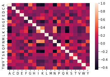
#correlation between different features 
sns.heatmap(df1.corr())

<AxesSubplot:>

Model building¶

Create data and label matrices.

df1_matrix = df1.iloc[:,range(20)].values ## X matrix
labels = df1.index.values ## Y matrix

Create training and testing datasets, build the model and check prediction accuracy.

# Split-out validation dataset"
validation_size = 0.20 # 20% data for testing
seed = None # change to int for reproducibility
X_train, X_validation, Y_train, Y_validation = model_selection.train_test_split(df1_matrix, labels, \
                                                                               test_size=validation_size, \
                                                                                random_state=seed)

new_clf = SVC()
model1 = new_clf.fit(X_train, Y_train)
Y_predicted = model1.predict(X_validation)
score1 = accuracy_score(Y_predicted, Y_validation)
print(score1)

0.8085106382978723

df1_matrix.shape

(234, 20)

Cross-validation¶

from sklearn.metrics import accuracy_score
from sklearn.svm import SVC

# Test options and evaluation metric
scoring = 'accuracy'

kfold = model_selection.KFold(n_splits=5)
cv_results = model_selection.cross_val_score(SVC(), df1_matrix, labels, cv=kfold, scoring=scoring)

print(cv_results)
print(cv_results.mean(), cv_results.std())

[0.38297872 0.34042553 0.65957447 0.34042553 0.30434783]
0.40555041628122107 0.12943119067958725

SVC().get_params()

{'C': 1.0,
 'break_ties': False,
 'cache_size': 200,
 'class_weight': None,
 'coef0': 0.0,
 'decision_function_shape': 'ovr',
 'degree': 3,
 'gamma': 'scale',
 'kernel': 'rbf',
 'max_iter': -1,
 'probability': False,
 'random_state': None,
 'shrinking': True,
 'tol': 0.001,
 'verbose': False}

Hyperparameters¶

clf_poly = SVC(kernel='poly', degree=3)
clf_rbf = SVC(kernel='rbf', C=10)

kfold = model_selection.KFold(n_splits=5)
cv_SVM_poly_results = model_selection.cross_val_score(clf_poly, df1_matrix, labels, cv=kfold, scoring=scoring)
cv_SVM_rbf_results = model_selection.cross_val_score(clf_rbf, df1_matrix, labels, cv=kfold, scoring=scoring)
print(cv_SVM_rbf_results)
print (cv_SVM_poly_results.mean(), cv_SVM_rbf_results.mean())

[0.70212766 0.65957447 0.78723404 0.5106383  0.65217391]
0.6281221091581869 0.6623496762257168

Grid Search¶

from sklearn.model_selection import GridSearchCV
tuned_parameters = [{'kernel': ['rbf'], 'gamma': [1e-3, 1e-4],
                     'C': [1, 10, 100, 1000, 10000]},
                    {'kernel': ['linear'], 'C': [1, 10, 100, 1000, 10000]},
                    {'kernel':['poly'], 'C': [1, 10, 100, 1000, 10000],
                     'degree': range(10)}]
clf_grid = GridSearchCV(SVC(), tuned_parameters, cv=5, scoring='accuracy')
clf_grid.fit(df1_matrix,labels)

GridSearchCV(cv=5, estimator=SVC(),
             param_grid=[{'C': [1, 10, 100, 1000, 10000],
                          'gamma': [0.001, 0.0001], 'kernel': ['rbf']},
                         {'C': [1, 10, 100, 1000, 10000], 'kernel': ['linear']},
                         {'C': [1, 10, 100, 1000, 10000],
                          'degree': range(0, 10), 'kernel': ['poly']}],
             scoring='accuracy')

print(clf_grid.best_params_)
#print(clf_grid.cv_results_)

{'C': 1, 'degree': 3, 'kernel': 'poly'}

Build a SVM model using above hyperparameters and check the prediction accuracy.

clf_poly = SVC(kernel='poly',C=1, degree=3)

kfold = model_selection.KFold(n_splits=5)
cv_SVM_results = model_selection.cross_val_score(clf_poly, df1_matrix, labels, cv=kfold, scoring=scoring)
print(cv_SVM_results)
print (cv_SVM_results.mean(),cv_SVM_results.std())

[0.70212766 0.65957447 0.76595745 0.40425532 0.60869565]
0.6281221091581869 0.12325451681757636

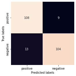
Confusion matrix¶

from collections import Counter
from sklearn.metrics import confusion_matrix

clf_new = SVC(kernel='poly',degree=3)

## Fit model to the data ##
clf_new.fit(df1_matrix,labels)
print(Counter(labels))

## Predict labels for the original data ##
clf_new_predict = clf_new.predict(df1_matrix)
print(Counter(clf_new_predict))

Counter({'1': 117, '-1': 117})
Counter({'-1': 121, '1': 113})

cm = confusion_matrix(labels,clf_new_predict)
print(cm)

fig,ax= plt.subplots()
sns.heatmap(cm, square=True, annot=True, fmt='g', cbar=False, ax=ax)
ax.set_xlabel('Predicted labels')
ax.set_ylabel('True labels')
ax.xaxis.set_ticklabels(['positive', 'negative'])
ax.yaxis.set_ticklabels(['positive', 'negative'])
plt.show()

[[108   9]
 [ 13 104]]

Exercise¶

Extract another feature - Di-Peptide Composition (DPC)

For each sequence calculate the frequency of pairwaise occurrence of amino acids. The length of the feature vector for each sequence would be 400 (20 x 20). Construct a classification model using DPC as a feature and compare the results with classification using amino acid composition.

import itertools
aa_list = ['A','C','D','E','F','G','H','I','K','L','M','N','P','Q','R','S','T','V','W','Y']

## Create a series of dipeptides
dpc_series = pd.Series(name='1',dtype=float)
for x in itertools.product(aa_list,aa_list):
    dpc_series[''.join([''.join(x)])] = 0

df_dpc = pd.DataFrame([])
for keys,values in positive_dict.items():
    dpc_series_copy = dpc_series.copy()
#    print (values.seq)
    dpc_seq = [str(values.seq[i:i+2]) for i in range(len(values.seq))]
    del dpc_seq[-1]
    for x in dpc_seq:
        dpc_series_copy[x] += 1
    dpc_series_copy /= len(values.seq)
    dpc_series_copy *= 100
    df_dpc = df_dpc.append(dpc_series_copy)
#dpc_series_copy

df_dpc

	AA	AC	AD	AE	AF	AG	AH	AI	AK	AL	...	YM	YN	YP	YQ	YR	YS	YT	YV	YW	YY
1	0.399202	0.000000	0.000000	0.399202	0.399202	0.399202	0.199601	0.199601	0.598802	0.199601	...	0.199601	0.000000	0.598802	0.199601	0.000000	0.199601	0.000000	0.000000	0.0	0.000000
1	1.345291	0.000000	0.149477	0.747384	0.149477	0.597907	0.149477	0.298954	0.896861	0.448430	...	0.000000	0.000000	0.298954	0.448430	0.000000	0.000000	0.298954	0.597907	0.0	0.000000
1	0.571429	0.000000	0.761905	0.761905	0.380952	1.142857	0.190476	0.380952	0.571429	1.142857	...	0.000000	0.000000	0.000000	0.000000	0.761905	0.190476	0.190476	0.190476	0.0	0.000000
1	0.331126	0.165563	0.331126	0.496689	0.662252	0.662252	0.331126	0.000000	0.165563	0.496689	...	0.000000	0.165563	0.165563	0.331126	0.827815	0.331126	0.000000	0.165563	0.0	0.000000
1	0.495050	0.000000	0.660066	0.990099	0.165017	0.660066	0.000000	0.165017	0.825083	0.825083	...	0.165017	0.495050	0.165017	0.165017	0.165017	0.165017	0.165017	0.330033	0.0	0.330033
...	...	...	...	...	...	...	...	...	...	...	...	...	...	...	...	...	...	...	...	...	...
1	0.790514	0.000000	0.592885	0.395257	0.592885	0.592885	0.197628	0.197628	1.185771	0.395257	...	0.000000	0.000000	0.197628	0.000000	0.395257	0.197628	0.000000	0.000000	0.0	0.000000
1	0.401606	0.000000	0.401606	0.200803	1.004016	0.200803	0.401606	0.000000	0.803213	0.200803	...	0.000000	0.000000	0.000000	0.401606	0.200803	0.602410	0.200803	0.803213	0.0	0.401606
1	2.923977	0.000000	1.754386	1.949318	1.169591	0.779727	0.194932	0.389864	0.000000	1.559454	...	0.000000	0.000000	0.194932	0.000000	0.584795	0.000000	0.000000	0.000000	0.0	0.000000
1	0.000000	0.000000	0.114416	0.114416	0.114416	0.114416	0.114416	0.114416	0.343249	0.114416	...	0.000000	0.228833	0.228833	0.000000	0.228833	0.228833	0.228833	0.228833	0.0	0.228833
1	0.000000	0.142653	0.285307	0.000000	0.570613	0.000000	0.285307	0.855920	0.570613	1.711840	...	0.000000	0.000000	0.142653	0.427960	0.000000	0.000000	0.142653	0.000000	0.0	0.285307

117 rows × 400 columns

Machine Learning